Optical density, normalization, and growth rates

Background on optical density

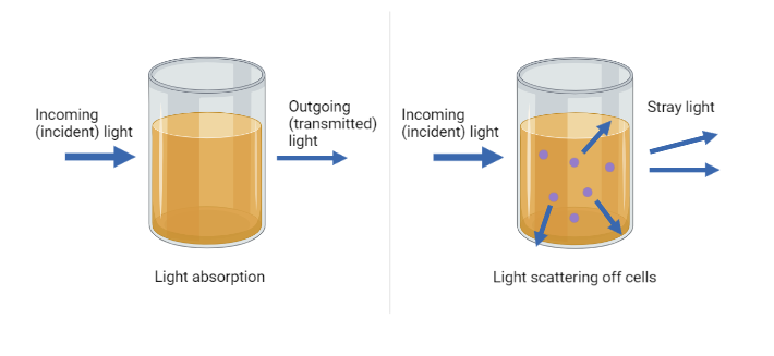
Light passing through a culture behaves differently than light passing through a clear solution. Instead of being absorbed, light is scattered by the cells in suspension. This scattered light is measured as optical density (OD). As turbidity increases, more scattering occurs, resulting in a higher OD reading.

tip

Looking to calibrate for OD600 readings? Visit this page.

Normalization

Due to manufacturing variation (LED strength and sensor sensitivity), raw OD readings can't be compared directly across devices. Instead, we use the normalization technique described below:

A series of initial OD readings are averaged to produce a reference value (baseline). New OD readings after the reference value are normalized using the following simple equation:

$$\frac{\normalsize \text{latest\thickspace OD}}{\normalsize \text{reference\thickspace OD}}=\text{normalized\thickspace OD}$$

For example:

Pioreactor name	Reference OD	Latest OD
Pioreactor1	0.030	0.033
Pioreactor2	0.010	0.015

It's difficult to compare raw OD readings since the starting values are different. However, if we normalize using the above equation:

Pioreactor1

$\frac{\small 0.033}{\small 0.030}=1.1$

Culture has grown by 1.1x.

Pioreactor2

$\frac{\small 0.015}{\small 0.010}=1.5$

Culture has grown by 1.5x.

We can more accurately compare culture growth using these ratios as opposed to using the raw OD values.

tip

Because of the way we defined normalized optical density, it has the following easy interpretation: it's the multiplicative amount the culture has changed by. So if the normalized OD is 2.0, the culture has doubled its initial concentration, i.e. doubled the population since the volume is fixed. This interpretation also maps to traditional OD600 measurements: if your initial sample has OD600 equal to 0.45, then a normalized OD of 2.0 is approximately an OD600 of twice that, or 0.90.

Blanking

While basic normalization accounts for initial OD differences, it does not consider the optical density of the media itself. For a more accurate growth rate calculation, you can blank your sample.

Blanking your vials is recommended for experiments that begin with low OD readings (e.g., inoculating small amounts of yeast). By blanking, you observe the OD of only the microorganism of interest.

As an example, let's consider the same data as above, but this time we have information on the blank ODs:

Pioreactor name	Blank OD (media)	Reference OD (media with culture)	Difference (reference - blank)	Latest OD
Pioreactor1	0.025	0.030	0.005	0.033
Pioreactor2	0.005	0.010	0.005	0.015

We can now subtract the blank values from both the latest OD and reference OD values:

$$\frac{\normalsize \text{latest\thickspace OD}-\text{blank\thickspace OD}}{\normalsize \text{reference\thickspace OD}-\text{blank\thickspace OD}}=\text{blanked\thickspace normalized\thickspace OD}$$

Pioreactor1

$\frac{\small 0.033-0.025}{\small 0.030-0.025}=1.6x$

Culture has grown by 1.6x.

Pioreactor2

$\frac{\small 0.015-0.005}{\small 0.010-0.005}=2x$

Culture has grown by 2x.

By accounting for the OD of the blank media, we are able to calculate a more accurate growth rate.

Growth rate

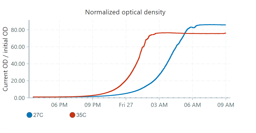
We inoculated two vials with a drop of re-hydrated yeast, and tracked their growth at temperatures 27°C and 35°C. The UI shows the following normalized optical density chart:

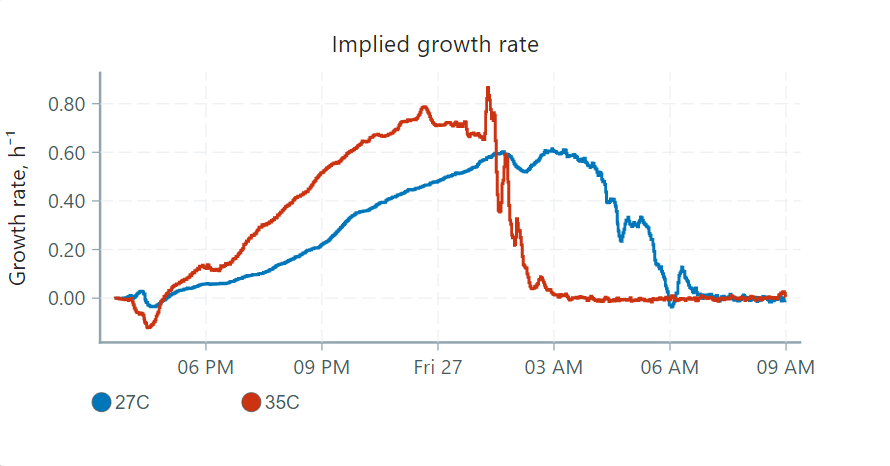
From normalized optical density, the UI also computes an implied growth rate. The relationship between the implied growth rate, $\text{gr}$, and the normalized optical density, $\text{nOD}$, is exponential and can be written as:

$$\text{nOD}(t) = \exp{ \left( \int_0^t \text{gr}(s)ds \right)}$$

We can rewrite this equation in terms of the growth rate:

$$\text{gr}(t)= \frac{ \text{nOD}'(t)} {\text{nOD}(t)}$$

This states that the growth rate is the rate of change of the culture size, normalized by the culture size.

This rate helps compare the state of your culture under different conditions (temperature, media, etc.).

These graphs can be interpreted in four phases:

• The lag phase: Little observed growth, but high cell activity. Cells acclimate to a nutrient-rich environment and prepare for division.
• Exponential (or log) phase: Cells divide and double at a roughly constant rate. Generation times depend on species and conditions.
• Stationary phase: Eventually the growth of cells reaches a plateau as nutrients are used up and waste products accumulate. At this point, the number of dividing cells will equal the number of dying cells.
• Decline (or death) phase: As nutrients are depleted, cell growth slows while cell death increases.

Here's how these phases would apply to our graphs, focusing on the 35°C vial:

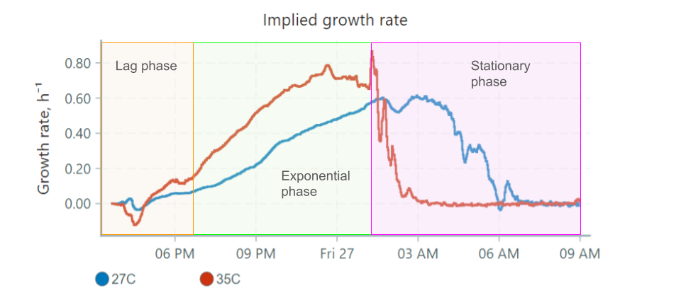
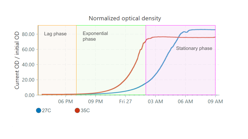
Some things to note:

• The lag phase can be detected easily in the growth rate graph, as the rate is stable and doesn't begin increasing until a bit after 6 PM. This is not easily determined in the nOD graph, since at this point the overall turbidity of the culture is low.
• The exponential phase occurs when the growth rate is high/increasing.
• When the culture reaches the stationary phase, growth rate drops to 0 since the culture is no longer growing in size. The turbidity is constant.
• The decline phase is not represented in the graphs above, as yeast remain in the stationary phase over many days.

(Optional) Blanking

When working with small amounts of a microorganism, or when using very turbid media, you can obtain more accurate growth rates by blanking the vial before inoculation.

How to record a blank #

1. Insert your sterile vial containing media into the Pioreactor before inoculating with your species of interest.
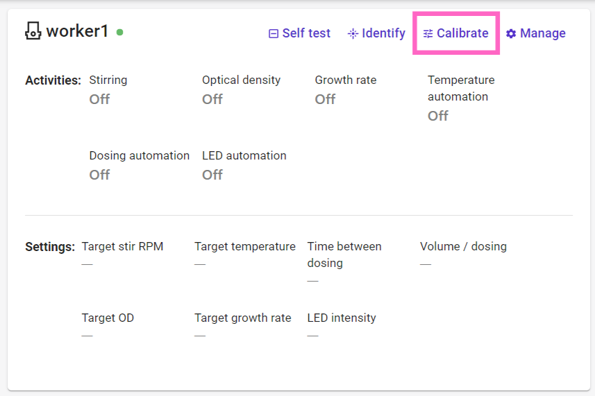
2. In the UI, click the Pioreactors tab on the left-hand menu, and choose one of the active pioreactors.
3. Select Calibrate, and under the Blanks tab, click Start. The Pioreactor will now record the optical density of the blank vial.
4. Repeat for all the Pioreactors to be used.
   • A notification will appear when a Pioreactor has finished blanking.
5. You can now inoculate your vials and begin your experiment.