Growth rate cuve modelling

Introduction to our growth-rate model

The study of the growth of bacterial cultures does not constitute a specialized subject or branch of research: it is the basic method of microbiology.” Monitoring and controlling the specific growth rate should not constitute a specialized subject or branch of research: it should be the basic method of advanced microbial bioprocessing. - Jacques Monod

The first step to controlling a culture's growth is to measure it. To do this, we need to model the rate of growth. We've seen other attempts at modelling the growth rate, but they all assumed too much:

• Exponential growth model: perhaps truly early on, but certainly not the case near stationary.
• Logistic growth model: requires an assumption about the max optical density, and assumes symmetric growth around the inflection point.
• Gompertz models and other models: more parameters, less interpretable, and still make strong assumptions about the trajectory of growth.

Further more, none of these can model a culture in a turbidostat or chemostat mode, where the optical density is dropping quickly during a dilution, but the growth rate should remain constant.

Re-visiting a growth model

We are often introduced to a growth model by the simple exponential growth model:

$\text{OD}(t) = \exp{\left( \text{gr} t \right)}$

Plainly put, the culture grows exponentially at rate $\text{gr}$. Like we mentioned above, this might be true for small time-scales, but certainly over the entire lag, log, and then stationary phases, this is not the case.

There's a hint of an interesting idea in the last paragraph though: "over small time scales". What if we cut up the growth curve into many small time intervals, and computed a growth rate for each interval? Then our growth rate can be changing: starts near 0 in the lag phase, can increase to a peak in the log phase, and then drop to 0 again in the stationary phase. We also don't need to assume any parametric form for the growth rate, we can just measure it directly from the data.

Our new formula might look like:

$\text{OD}(t) = \exp{\left(\text{gr}_0 \Delta t + \text{gr}_1 \Delta t + ... \right)}$

If we think more about this, and we keep shrinking our time interval towards zero, this is just an integral:

$$\text{nOD}(t) = \exp{ \left( \int_0^t \text{gr}(s)ds \right)}$$

There's still no particular assumption about the shape of the growth rate function, $gr(s)$. For example, consider the following ODs from a batch experiment:

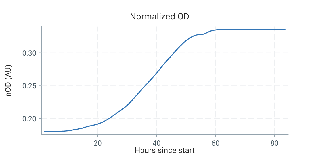
Using our estimation technique outlined below, we can estimate the growth curve as:

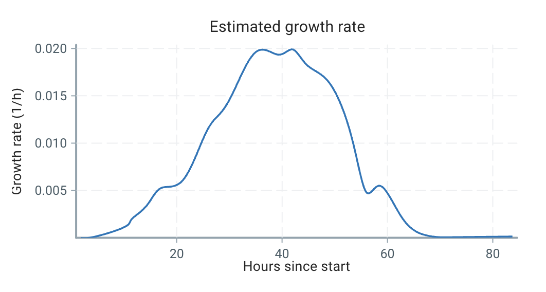
We can see that the growth is very dynamic, and certainly not a single number or a constrained form!

Estimating a non-parametric growth rate

A non-parametric, dynamic growth rate sounds great, but we've replaced a estimation of a single value (or handle of values) to an entire function! This seems expensive!

Luckily, we do the work for you. We will compute $gr(t)$ using a statistical algorithm, the Kalman filter. The Kalman filter is an algorithm that estimates the state of a dynamic system from noisy measurements. In our case, the state is the growth rate, and the measurements are the optical density readings. We input optical density observations one at a time, and the Kalman filter updates its estimate of the growth rate based on the new observation. This allows us to track the growth rate in real-time, as the culture grows.

Online: Using the Pioreactor's software

When you start the "Growth rate" action in your Pioreactor, the action starts reading from the stream of OD readings, and computes the growth-rate for each reading. The growth rate is then displayed in the Pioreactor UI.

Offline: Using the growth-rate tool

We have implemented our algorithm and estimation in an easy-to-use web app, the growth-rate tool. You can use this tool to upload your optical density and (optionally) dosing events data, and it will compute the growth rate for you.

Backed by our Python library, grpredict

If you want more control, you can use our grpredict Python library, available with:

pip install grpredict

This is the same library that's used in our Pioreactor software.

Model parameters

• baseline samples: the number of samples at the start of the dataset to use for initial variance calculations, and as the baseline value to normalize the optical densities against (so that the initial nOD is nearly equal to 1.0)
• Growth-rate std: a Kalman-filter specific parameter. Higher values allow more flexibility in the growth rate, lower values smooth the growth rate.
• nOD std.: a Kalman-filter specific parameter. If your dosing large amounts at a time, you may want to increase this.
• OD std. factor: a Kalman-filter specific parameter. If your sample are very noisy, you can increase 2x to dampen the affect of that noise.
• Outlier threshold: a Kalman-filter specific parameter. Large outliers or shifts in OD will likely be taken care of by setting this to 5, but try values between 3 and 5 if you want to handle less large outliers.

Required CSV schemas for growth-rate tool

To upload your optical density and dosing events data to the Pioreactor, you need to prepare CSV files with specific schemas. Below are the required formats for each file, along with common pitfalls to avoid.

tip

If using the Pioreactor UI to export datasets Optical density and Dosing event log, these already have the correct schema.

1. Optical-Density CSV

Column	Required?	Expected dtype	Description
od_reading	Yes	float	Raw or pre-normalized optical-density measurement.
hours_since_experiment_created	Yes	float	Elapsed hours since the experiment’s “time 0”. Use decimals for sub-hour resolution (e.g. 0.4167 ≈ 25 min).
pioreactor_unit	No	string	use this column to partition different experiments or units

info

Additional columns (sensor angle, experiment name, etc.) are ignored by the parser, so feel free to keep them.

Minimal example

od_reading,hours_since_experiment_created
0.1725,0.397
0.1735,0.399
0.1749,0.402

Multiple units example

pioreactor_unit,od_reading,hours_since_experiment_created
A,0.1725,0.397
A,0.1735,0.399
B,0.1249,0.397
B,0.1280,0.399

---

2. Dosing-events CSV

Column	Required?	Expected dtype	Description
event	Yes	category (string)	Either add_media, add_alt_media, or remove_waste.
volume_change_ml	Yes	float	volume change (mL)
hours_since_experiment_created	Yes	float	Timestamp in hours, exactly matching the OD clock.
pioreactor_unit	No	string	use this column to partition different experiments or units

Minimal example

event,volume_change_ml,hours_since_experiment_created
add_media,1.0,1.533
remove_waste,1.0,1.544
remove_waste,2.0,1.567

---

Common pitfalls

• Header spelling matters – odReading, OD_reading, or trailing spaces will fail validation.
• Mixed delimiters – Ensure you’re saving with commas.
• Units – volume_change_ml must be millilitres; convert L → mL beforehand.
• Consistent clock – Both files must use the same hours_since_experiment_created reference, or dilution jumps won’t align.